Create a config.ini
Generate default values
In most case, whether you’re new to ForMoSA or not, we strongly recommend using this method to generate your first config file.
Download this empty config file : config.ini 📥.
Set up your paths (i.e., tell ForMoSA where to find the data and model files, and where to store the results).
Launch
global_file.pywith this config file. This will automatically create a reference config file (config_ref.ini) inresult_pathwith all missing inputs; i.e. :
[1]:
from ForMoSA.global_file import GlobFile
config_path = '/home/mravet/Documents/These/FORMOSA/OUTPUTS/Channel1/config.ini'
GlobFile(config_path) # => Will create a complete config file with all default values
---------------------------------------------------------------------------
ModuleNotFoundError                       Traceback (most recent call last)
Cell In[1], line 1
----> 1 from ForMoSA.global_file import GlobFile
      2 config_path = '/home/mravet/Documents/These/FORMOSA/OUTPUTS/Channel1/config.ini'
      3 GlobFile(config_path) # => Will create a complete config file with all default values

ModuleNotFoundError: No module named 'ForMoSA'
You can now modify
config_ref.iniwith the parameters you want ! Be careful : you must at least define the prior values for the grid parameters before running an inversion. Check next section to learn more about each parameters.
Why bother with this ?
In future updates, some parameters may be added or removed. Generating a new config ensures that you’ll always have access to all available parameters provided by ForMoSA ☺️ !
Parameters (version 1.1.6)
List and description of each config file parameter. If, for a given parameter, ‘MOSAIC : Yes’, it means that the parameter can be defined separatly for each observation (i.e parameter = par1, par2, …)
[config_adapt]
method= Interpolation method for the grid.format :
'linear'or'nearest'or'zero'or'slinear'or'quadratic'or'cubic'or'quintic'or'pchip'or'barycentric'or'krogh'or'akima'or'makima'comments :
'linear'will be used by default. ⚠️ For safety reasons, this will also be the interpolation method during the nested sampling. Refer to the xarray documentation for more details.MOSAIC : No
emulator= Emulator to use.format :
'NA'or'PCA', ncompor'NMF', ncompcomments :
'NA'will be used by default, meaning the grid won’t be emulated.ncompis the number of components used for the PCA or NMF decomposition. ⚠️ You cannot set more components than the number of spectral channels. Refer to the scikit-learn documentation for more details.MOSAIC : No (will soon change)
target_res_obs= Observation resolution to reach.format :
'obs'orfloatcomments :
'obs'will be used by default, meaning ForMoSA won’t change the observation resolution. If a float is given, ForMoSA will take the minimum between this value, the resolution of the model and the resolution of the observation.MOSAIC : Yes
target_res_mod= Model resolution to reach (prior to the inversion).format :
'obs'or'mod'orfloatcomments :
'obs'will be used by default, meaning ForMoSA will convolve and resample the model to the observation resolution prior to the inversion. If'mod', ForMoSA won’t change the model resolution prior to the inversion (usefull for high resolution spectroscopy). If a float is given, ForMoSA will take the minimum between this value and the resolution of the model.MOSAIC : Yes
res_cont= Approximate resolution of the continuum.format :
'NA'orfloatcomments :
'NA'will be used by default, meaning ForMoSA won’t remove the continuum. If a float is given, ForMoSA will remove a continuum extracted at this resolution. ⚠️ To use this parameter, you must also definewav_cont(see below).MOSAIC : Yes
wav_cont= Wavelength range(s) used to estimate of the continuum.format :
'NA'or'window1_min / window1_max, window2_min / ... / windowN_max'comments :
'NA'will be used by default, meaning ForMoSA won’t remove the continuum. If a wavelength range (in µm) is provided, ForMoSA will remove a continuum estimated using this range. ⚠️ To use this parameter, you must also defineres_cont(see above). Separate windows can be defined using'/'as separator.MOSAIC : Yes
[config_inversion]
logL_type= Log-likelihood used during inversion.format :
'chi2'or'chi2_covariance'or'chi2_noisescaling'or'chi2_noisescaling_covariance'or'CCF_Brogi'or'CCF_Zucker'or'CCF_custom'comments :
'chi2'will be used by default. This defines the core of the inversion. The choice of likelihood function entirely depends on the type of data you’re dealing with. ⚠️ Photometric points are always compared to the model using'chi2', regardless of the likelihood selected for spectroscopy.MOSAIC : Yes
exemple:
'chi2' : \(~~~log(L)=-\frac{\chi^2}{2}=-\frac{1}{2}\sum\left(\frac{d-m}{\sigma}\right)^2\)
'chi2_covariance' : \(~~~log(L)=-\frac{\chi^2}{2}=-\frac{1}{2}(d-m)^T C^{-1} (d-m)\)
'chi2_noisescaling' : \(~~~log(L)=-\frac{N}{2}log\left(\frac{\chi^2}{N}\right)=-\frac{N}{2}log\left(\sum\frac{1}{N}\left(\frac{d-m}{\sigma}\right)^2\right)\) Ruffio et al. (2019)
'chi2_noisescaling_covariance' : \(~~~log(L)=-\frac{N}{2}log\left(\frac{\chi^2}{N}\right)=-\frac{N}{2}log\left(\frac{1}{N}(d-m)^T C^{-1} (d-m)\right)\) Ruffio et al. (2019)
'CCF_Brogi' : \(~~~log(L)=-\frac{1}{2}log\left(S_f^2 + S_m^2 - 2R\right)=-\frac{1}{2}log\left(\frac{1}{N}\sum d^2 + \frac{1}{N}\sum m^2 - 2\frac{1}{N}\sum dm \right)\) Brogi et al. (2019)
'CCF_Zucker' : \(~~~log(L)=-\frac{1}{2}log\left(1 - C^2\right)=-\frac{1}{2}log\left(1 - \frac{\sum dm}{\sum d^2 \sum m²}\right)\) Zucker et al. (2003)
'CCF_custom' : \(~~~log(L)=-\frac{1}{2\bar\sigma}\left(S_f^2 + S_m^2 - 2R\right)=-\frac{1}{2} \left(\frac{1}{N}\sum\frac{1}{\sigma^2} \right) \left(\frac{1}{N}\sum d^2 + \frac{1}{N}\sum m^2 - 2\frac{1}{N}\sum dm \right)\)
… with \(d\) and \(m\) being the data and model arrays, respectively. \(\sigma\) represents the error bars, and \(C\) is the covariance matrix.
logL_full= If you want to use the full loglikelihood during the inversion.format :
'True'or'False'comments :
'False'will be used by default. This means that the constant terms: \(-\frac{N}{2} log(2\pi) - \frac{1}{2} log(|C|)\) will be ignored.MOSAIC : Yes
exemple:
wav_fit= Wavelength range(s) used during the nested sampling procedure.format :
'window1_min / window1_max, window2_min / ... / windowN_max'comments :
'0,100'will be used by default. If a wavelength range (in µm) is provided, ForMoSA will ignore all points outside of it during the inversion. Separate windows can be defined using'/'as separator.MOSAIC : Yes
ns_algo= Nested sampling algorithm.format :
'nestle'or'pymultinest'or'ultranest'comments :
'nestle'will be used by default. We recommend using'pymultinest'for large datasets as it enables for efficient parallelisation. Refer to nestle, pymultinest and ultranest documentations for more details.MOSAIC : No
npoint= Number of living points during the nested sampling procedure.format :
intcomments :
100will be used by default.MOSAIC : No
[config_highcont_models]
hc_type= Method to compute the high-contrast model.format :
'NA'or'nofit_rm_spec'or'nonlinear_fit_spec'or'fit_spec'or'rm_spec'or'fit_spec_rm_cont'or'fit_spec_fit_cont'comments :
'NA'will be used by default, meaning ForMoSA won’t fit for stellar contamination. This defines the function used to compute the high-contrast model. ⚠️ To use this parameter, you must also definehc_bound_lsq(see below). We strongly recommend that new users read the API documentation on high-contrast models before using these functions.MOSAIC : Yes
hc_bounds_lsq= Least-square bounds.format :
'NA'or'lower, upper'comments :
'NA'will be used by default, meaning ForMoSA won’t fit for stellar contamination. This defines the bounds of the lsq used to compute the high-contrast model. ⚠️ To use this parameter, you must also definehc_bound_lsq(see below). We strongly recommend that new users read the API documentation on high-contrast models before using these functions.MOSAIC : Yes
[config_parameters]
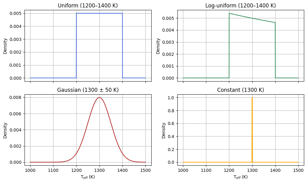
This is where physics happens ! 😊. You’ll be able to define priors and ranges for your physical parameters.
As of now, four functions can be used :
'uniform', lower, upper'loguniform', lower, uppper(⚠️loweranduppermust be >0)'gaussian', mu, sigma'constant', value
⚠️ For parameters available with MOSAIC, you should ALWAYS use three entries per observation (e.g. prior_1, value1_1, value2_1, prior_2, value1_2, value2_2, …, prior_N, value1_N, value2_N)
parN= N’th (from 1 up to 5) parameter of the atmospheric grid.format :
'NA'or'prior', value1, value2comments :
'NA'will be used by default. These are the main parameters of your inversion. They are specific to each atmospheric grid, but usually include quantities like \(T_{eff}\), \(log(g)\), \([M/H]\), … ⚠️ Be sure to check the documentation of the grid to learn the number of parameters and their valid ranges.MOSAIC : No
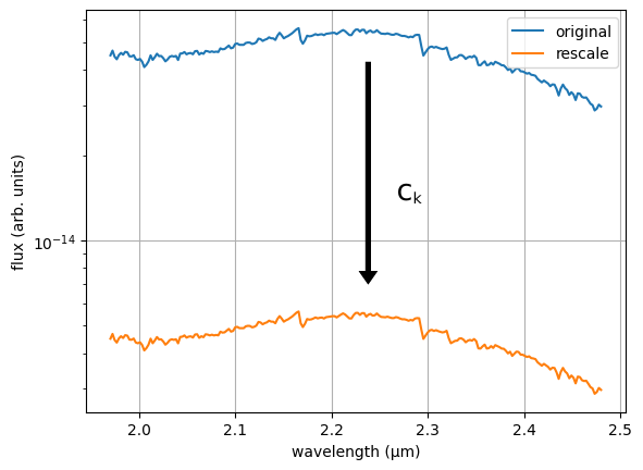
r= Radius in \(R_{jup}\).format :
'NA'or'prior', value1, value2comments :
'NA'will be used by default, meaning ForMoSA will do an analytical rescaling. You need to define bothranddso that ForMoSA can compute an analytical scaling factorck=(r/d)²to rescale the model. ⚠️ This parameter cannot be used alongside high-contrast models, as they also apply a rescaling to the model.MOSAIC : No
d= Distance in \(pc\).format :
'NA'or'prior', value1, value2comments :
'NA'will be used by default,meaning will do an analytical rescaling. You need to define bothranddso that ForMoSA can compute an analytical scaling factorck=(r/d)²to rescale the model. ⚠️ This parameter cannot be used alongside high-contrast models, as they also apply a rescaling to the model.MOSAIC : No
alpha= Scaling parameter.format :
'NA'or'prior', value1, value2comments :
'NA'will be used by default, meaningalpha=1. You need to define bothranddso that ForMoSA can compute an analytical scaling factorck=alpha*(r/d)²to rescale the model. ⚠️ This parameter cannot be used alongside high-contrast models, as they also apply a rescaling to the model. We also strongly recommend that you put constraining priors on this parameter as it is highly degenerated with bothrandd. If you have multiple observations and fit multiplealphas, setting one of them to'NA'will use the analytical computation of the scaling factor (usefull for continuum-substracted data).MOSAIC : Yes
exemple :
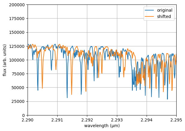
rv= Radial velocity in \(km/s\).format :
'NA'or'prior', value1, value2comments :
'NA'will be used by default. This parameter shifts the model in wavelength. To avoid edge effects during reinterpolation, iftarget_res_mod = 'mod'ortarget_res_mod = float, the model is saved with a larger spectral extent during the adaptation step.MOSAIC : Yes
exemple :
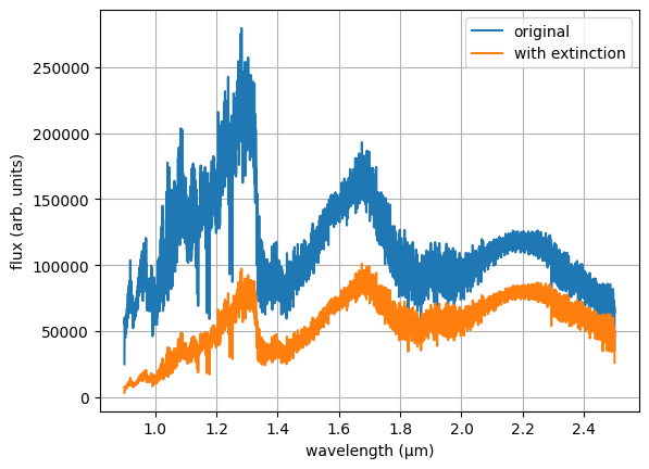
av= Extinction coeficient in \(mag\).format :
'NA'or'prior', value1, value2comments :
'NA'will be used by default. This will apply interstellar extinction to the model. It can also be used to emulate missing cloud opacities in your grid.MOSAIC : No
exemple :
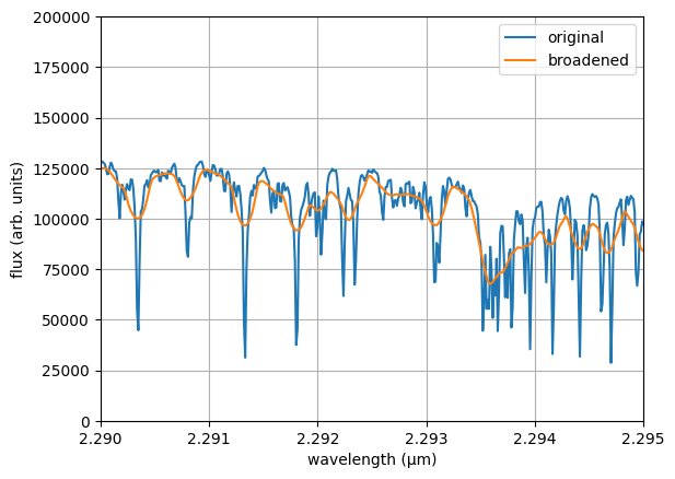
vsini= Projected rotational velocity in \(km/s\).format :
'NA'or'prior', value1, value2, 'method'comments :
'NA'will be used by default. You need to define bothvsiniandldso that ForMoSA can compute the broadening of the spectral lines. Constraints obtained on this parameter for observations at a resolution $<$100,000 are not robust for slow rotators. To avoid edge effects during reinterpolation, we also recommend to fitrvas well. Since this parameter can be computationally expensive to fit, ForMoSA allows you to choose between four methods :'RotBroad'or'FastRotBroad'or'Accurate'or'AccurateFastRotBroad'. You should always specify your method after the priors. Please refer to the API documentation for more information.MOSAIC : Yes
ld= Limb-darkening.format :
'NA'or'prior', value1, value2comments :
'NA'will be used by default. You need to define bothvsiniandldso that ForMoSA can compute the broadening of the spectral lines. This parameter is usually hard to constrain so we recommend using a constant value.MOSAIC : Yes
exemple :
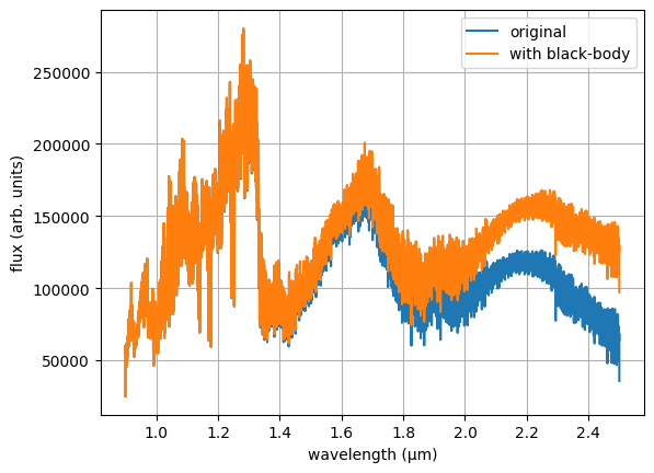
bb_t= Black-body temperature in \(K\).format :
'NA'or'prior', value1, value2comments :
'NA'will be used by default. You need to definebb_t,bb_randdso that ForMoSA can add the contribution from a simple black-body circumplanetary disk.MOSAIC : No
bb_r= Black-body radius in \(R_{jup}\).format :
'NA'or'prior', value1, value2comments :
'NA'will be used by default. You need to definebb_t,bb_randdso that ForMoSA can add the contribution from a simple black-body circumplanetary disk.MOSAIC : No
[config_nestle]
See Nestle documentation
[config_pymultinest]
See Pymultinest documentation
[config_ultranest]
See Ultranest documentation