Knowing the Config#

ForMoSA is controlled through a set of Python dataclasses — one for each concern. You can either instantiate them directly in code (preferred) or load them from an INI file.

Two ways to configure#

Option A — Python dataclasses (recommended)#

from ForMoSA import Analysis
from ForMoSA.config.global_config import (
    ConfigPath, ConfigAdapt, ConfigInversion, ConfigParameters
)

config_path = ConfigPath(
    observation_path  = ["data/obs.fits"],
    adapt_store_path  = "adapted_grid/",
    result_path       = "results/",
    model_path        = "atm_grids/BT-Settl.nc",
)
config_adapt      = ConfigAdapt()
config_inversion  = ConfigInversion(ns_algo="pymultinest", npoints=200)
config_parameters = ConfigParameters(
    par1=["uniform", "500",  "3000"],   # Teff
    par2=["uniform", "2.5",  "5.5"],    # log g
    r   =["uniform", "0.5",  "3.0"],    # radius (R_Jup)
    d   =["constant", "50"],            # distance (pc)
)

analysis = Analysis(config_path)
analysis.adapt(config_adapt, config_inversion)
analysis.nested_sampling(config_parameters, config_adapt, config_inversion)
analysis.plot(analysis.ns.results)

Option B — INI file#

[ConfigPath]
observation_path = data/obs.fits
adapt_store_path = adapted_grid/
result_path      = results/
model_path       = atm_grids/BT-Settl.nc

[ConfigInversion]
ns_algo  = pymultinest
npoints  = 200

[ConfigParameters]
par1 = uniform, 500, 3000
par2 = uniform, 2.5, 5.5
r    = uniform, 0.5, 3.0
d    = constant, 50

Load it with:

from ForMoSA.config.global_config import ConfigLoader

loader = ConfigLoader("config.ini")
config_path, config_adapt, config_inversion, config_parameters = loader.load()

Generate a template INI file with:

from ForMoSA.config.global_config import ConfigGenerator
ConfigGenerator().save("config_template.ini")

Which dataclass controls what#

Dataclass	Controls
`ConfigPath`	File paths: observations, model grid, adapted sub-grids, results
`ConfigAdapt`	Grid adaptation: interpolation method, resolution targets, continuum removal, parallelisation
`ConfigInversion`	Nested sampling: algorithm choice, live points, likelihood type, fitting wavelength range
`ConfigParameters`	Prior distributions for each fitted parameter

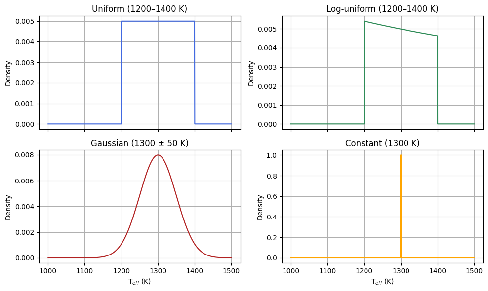
Prior syntax#

Every parameter in ConfigParameters accepts a list in the form:

["prior_type", "arg1", "arg2"]

Prior type	Syntax	Description
`uniform`	`["uniform", "min", "max"]`	Flat prior between min and max
`log_uniform`	`["log_uniform", "min", "max"]`	Flat in log-space
`gaussian`	`["gaussian", "mean", "std"]`	Normal distribution
`constant`	`["constant", "value"]`	Fixed value, not sampled
`NA`	`["NA"]`	Parameter disabled

Plot of different priors

Mode validity matrix#

The table below shows which parameters are relevant in each analysis mode. Parameters marked “No” will be ignored if provided but are not required.

Parameter	Standard	MOSAIC	Photometry-only	HCHR
`par1`–`par4`	Yes	Yes	Yes	Yes
`r`	Yes	Yes	Yes	No
`d`	Yes	Yes	Yes	No
`rv`	Yes	Yes	No	Yes
`vsini`	Yes	Yes	No	Yes
`ld`	Yes	Yes	No	Yes
`alpha`	Yes	Yes	Yes	No
`bb_T`	Yes	Yes	No	No

In MOSAIC mode, any parameter can be made instrument-local by appending its observation index: rv_0, rv_1, alpha_2, etc. Global parameters (without a suffix) are shared across all instruments.

Parameter reference#

`[ConfigPath]`#

observation_path (list of str or Path) : Paths to your .fits observation files. Single observation: one-element list. MOSAIC mode: one entry per instrument.

adapt_store_path (str or Path) : Directory where adapted sub-grids are saved. Shared across targets in the same sample (see Folder Structure).

result_path (str or Path) : Directory where ForMoSA writes results: ns_results.json, plots, saved observation state.

model_path (str or Path) : Path to the .nc model grid file.

`[ConfigAdapt]`#

method (str, default "linear") : Interpolation method used to resample the model grid onto the observation wavelength grid. "linear" is robust for most cases.

target_res_obs (list, default ["obs"]) : Target spectral resolution for each observation. "obs" uses the native observation resolution. Provide a float to force a specific resolution. One value per observation in MOSAIC mode (or a single value broadcast to all).

target_res_mod (list, default ["obs"]) : Target wavelength and resolution for the adapted sub-grid. "obs" uses the observation wavelength grid; "mod" keeps the native model grid.

wav_cont (list, default ["NA"]) : Wavelength ranges (in µm) used for continuum estimation and removal. Format: ["1.0, 1.3", "1.5, 1.8"]. "NA" disables continuum removal.

res_cont (list, default ["NA"]) : Spectral resolution used for the continuum estimate. Must match wav_cont in length. "NA" uses the native grid resolution.

backend (str, default "loky") : joblib parallelisation backend for grid adaptation. Options: "loky", "multiprocessing", "threading", "sequential", "dask", "ray". Use "sequential" to disable parallelisation for debugging.

n_jobs (int, default -1) : Number of parallel workers. -1 uses all available CPUs.

`[ConfigInversion]`#

ns_algo (str, default "pymultinest") : Nested-sampling back-end. Options: "pymultinest", "nestle", "ultranest". PyMultiNest is recommended for fits with more than three free parameters.

npoints (int, default 50) : Number of live points. More points → better posterior sampling and evidence estimate, but longer run time. Start with 50–100 for testing; use 300–500 for publication-quality runs.

logL_type (list, default ["chi2"]) : Log-likelihood function. Options: "chi2", "chi2_covariance", "chi2_noisescaling", "chi2_noisescaling_covariance", "CCF_Zucker", "CCF_Brogi", "CCF_custom". One value per observation in MOSAIC mode (or broadcast).

Log-likelihood equations and when to use each#

Let \(\Delta f_i = f_i^{\rm obs} - f_i^{\rm mod}\) be the residual at wavelength point \(i\), \(\sigma_i\) the 1-σ uncertainty, \(\mathbf{C}\) the covariance matrix, and \(N\) the number of data points.

chi2 — standard χ²

\[ \ln\mathcal{L} = -\frac{1}{2} \sum_{i=1}^{N} \left(\frac{\Delta f_i}{\sigma_i}\right)^2 \]

Assumes Gaussian, spectrally uncorrelated noise with well-calibrated uncertainties. Use when: your error bars are reliable and the noise is pixel-independent (e.g. photon-noise dominated spectra where the pipeline correctly propagates errors).

chi2_covariance — generalised χ² with a covariance matrix

\[ \ln\mathcal{L} = -\frac{1}{2}\, \boldsymbol{\Delta f}^{\!\top} \mathbf{C}^{-1} \boldsymbol{\Delta f} \]

Accounts for correlated noise between wavelength channels (e.g. from spline-based continuum removal, interpolation, or detector persistence). Use when: you have a full covariance matrix in the COVARIANCE FITS extension. Computationally more expensive than chi2.

chi2_noisescaling — χ² with marginalised noise-scaling

\[ \ln\mathcal{L} = -\frac{N}{2} \ln\!\left(\frac{1}{N}\sum_{i=1}^{N}\left(\frac{\Delta f_i}{\sigma_i}\right)^2\right) \]

Marginalises analytically over a global noise-scaling factor \(s\) (i.e. assumes the true noise is \(s \cdot \sigma_i\) for some unknown \(s\)). This makes the likelihood robust to a systematic over- or under-estimation of the error bars. Use when: you distrust the absolute scale of your uncertainties but believe their relative values (shape) are correct. Recommended default for medium-resolution ground-based spectra where sky-subtraction residuals inflate errors unevenly.

chi2_noisescaling_covariance — generalised χ² with marginalised noise-scaling

\[ \ln\mathcal{L} = -\frac{N}{2} \ln\!\left(\frac{1}{N}\, \boldsymbol{\Delta f}^{\!\top} \mathbf{C}^{-1} \boldsymbol{\Delta f}\right) \]

Combines the covariance matrix and noise-scaling marginalisation. Use when: you have correlated noise and uncertain absolute error scaling.

CCF_Brogi — cross-correlation log-likelihood (Brogi & Line 2019)

\[ \ln\mathcal{L} = -\frac{N}{2} \ln\!\left(\langle f^2\rangle - 2\langle f \cdot g\rangle + \langle g^2\rangle\right) \]

where \(f\) and \(g\) are the mean-subtracted observed and model spectra, and \(\langle \cdot \rangle\) denotes the mean over wavelength points. Use when: the absolute flux level is unknown or poorly calibrated (e.g. high-contrast residual spectra after speckle subtraction). The CCF-based likelihood is insensitive to multiplicative continuum offsets.

CCF_Zucker — cross-correlation log-likelihood (Zucker 2003)

\[ \ln\mathcal{L} = -\frac{N}{2} \ln\!\left(1 - \frac{\langle f g\rangle^2}{\langle f^2\rangle \langle g^2\rangle}\right) \]

Related to CCF_Brogi but normalised by the individual variances, making it equivalent to the Pearson correlation coefficient. Use when: similar to CCF_Brogi. Tends to be slightly more conservative (flatter posterior) near the peak. Prefer CCF_Brogi in most cases.

CCF_custom — noise-weighted cross-correlation

\[ \ln\mathcal{L} = -\frac{N}{2\sigma^2_w}\left(\langle f^2\rangle + \langle g^2\rangle - 2\langle fg\rangle\right) \]

where \(\sigma^2_w = \left(\frac{1}{N}\sum_i \sigma_i^{-2}\right)^{-1}\) is the harmonic-mean noise variance. Use when: you have per-pixel uncertainties and want a CCF-style likelihood that down-weights noisy channels. Bridges chi2_noisescaling and CCF_Brogi.

Tip

Quick decision guide:

Well-calibrated errors, no correlated noise → chi2
Uncertain absolute error scale → chi2_noisescaling (recommended default for most ground-based spectra)
Known correlated noise (covariance matrix available) → chi2_covariance
Continuum-subtracted or speckle-dominated spectra (HCHR) → CCF_Brogi
MOSAIC with mixed instruments → mix logL types, e.g. ["chi2_noisescaling", "CCF_Brogi"]

wav_fit (list, default ["0.9, 5.0"]) : Wavelength range (µm) used for the likelihood evaluation. Syntax: ["min, max"]. Points outside this range are masked. One value per observation in MOSAIC mode.

hc_lower_bounds_lsq / hc_higher_bounds_lsq (list, default ["NA"]) : Lower and upper bounds for the least-squares optimisation in HCHR mode. "NA" means unbounded. These are only relevant when the observation file has STAR_FLX.

`[ConfigParameters]` — fitted parameters#

All parameters share the same prior syntax: ["prior_type", "arg1", "arg2"]. Set to ["NA"] to disable.

par1, par2, par3, par4 — grid parameters : The physical parameters of the atmospheric model grid. What they represent depends on the grid (e.g. for BT-Settl: par1 = T_eff in K, par2 = log g). Check your grid’s documentation or inspect the coordinate names with xarray.

r — radius (R_Jup) : Companion radius. Used in the physical flux scaling: flux_obs = flux_model × (r / d)². Requires d to be set. Prior example: ["uniform", "0.5", "3.0"].

d — distance (pc) : Distance to the system. Usually fixed to the Gaia/Hipparcos value. Example: ["constant", "50"].

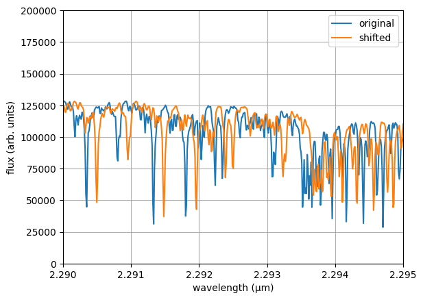
rv — radial velocity (km/s) : Doppler shift applied to the model spectrum before comparison. Not applicable to photometry-only observations.

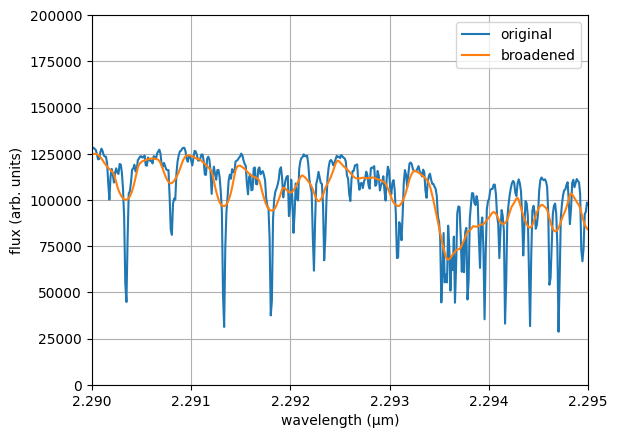
Radial velocity shift applied to model spectrum

vsini — rotational broadening (km/s) : Rotational broadening applied to the model via a convolution kernel. Requires specifying the kernel function as a fourth element: ["uniform", "0", "100", "FastRotBroad"]. You need to define both vsini and ld so that ForMoSA can compute the broadening of the spectral lines. Constraints obtained on this parameter for observations at a resolution <100,000 are not robust for slow rotators. To avoid edge effects during reinterpolation, we also recommend to fit rv as well. Since this parameter can be computationally expensive to fit, ForMoSA allows you to choose between four methods : RotBroad or FastRotBroad or Accurate or AccurateFastRotBroad. You should always specify your method after the priors. Please refer to the API documentation for more information.

Rotational broadnening applied to model spectrum

ld — limb-darkening coefficient : Linear limb-darkening coefficient applied to the model before scaling. Spectroscopic mode only.

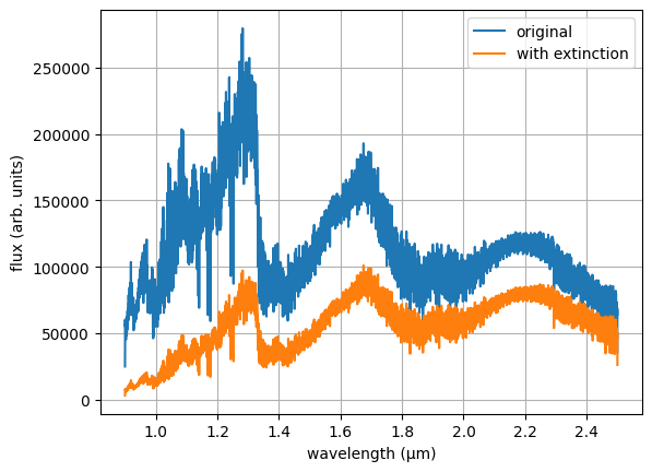
av — dust extinction (magnitudes) : ISM-like dust extinction applied to the model spectrum using the Cardelli (1989) extinction law with R_V = 3.1. The value is in V-band magnitudes (A_V). Useful when the companion is seen through significant foreground or circumstellar dust. Prior example: ["uniform", "0", "10"].

Extinction applied to model spectrum

alpha — analytical scaling factor : Multiplies the model flux by a constant: flux_obs = flux_model × α. Use instead of r+d when you do not want to constrain the radius. See Analytical vs Physical Scaling.

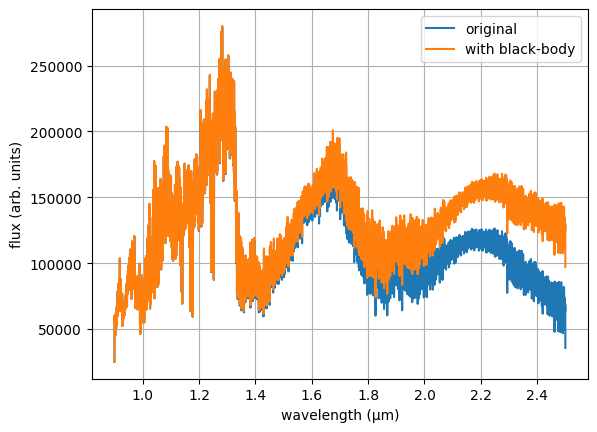
bb_T — blackbody component temperature (K) : Adds a Planck blackbody spectrum at temperature bb_T scaled by radius bb_R to the model spectrum. Useful when modelling a circumplanetary disk contribution, a thermal excess from a hot inner disk, or a secondary stellar component. Must be used together with bb_R. Prior example: ["uniform", "500", "3000"].

bb_R — blackbody component radius (R_Jup) : Effective radius of the blackbody component added by bb_T. Scales the blackbody flux so that bb_flux = Planck(bb_T) × (bb_R / d)². Prior example: ["uniform", "0.1", "5.0"].

Blackbody component added to model spectrum