
Tutorial 1 — Photometry: VHS 1256 b#
What you’ll learn: How to run a photometric atmosphere retrieval with ForMoSA v2.0 — loading multi-instrument broadband photometry, configuring the analysis with Python dataclasses, adapting a model grid, running nested sampling, and interpreting the results.
Target: VHS J125601.92−125723.9 b (VHS 1256 b) — a ~140 Myr, planetary-mass companion at ~22 pc with one of the most extreme red colours of any directly-imaged companion known. It sits on the L/T transition and hosts a spectrum dominated by thick, silicate clouds. It has been observed by SPHERE and NACO at the VLT, and more recently by JWST/NIRCam and JWST/MIRI.
Data: 14 broadband photometric points spanning 1–16 µm (SPHERE + NACO + JWST NIRCam + JWST MIRI).
Grid: BT-Settl (Allard et al. 2012) — Teff: 1000–3000 K, log g: 2.5–5.5
Estimated runtime:
Grid adaptation: ~ 5 min
Nested sampling (100 live points, nestle): ~15 min
References: Miles et al. (2023); Petrus et al. (2024)
Section 0: Setup#
Run these four cells before anything else. They check your environment, create the working directories, download the observation data, and download the model grid.
[1]:
# Environment check
import sys

try:
    import ForMoSA
    print(f"ForMoSA {ForMoSA.__version__} — OK")
except ImportError:
    raise ImportError(
        "ForMoSA is not installed.\n"
        "Run:  pip install ForMoSA && conda install dask netCDF4 bottleneck"
        "or: install from source:  git clone https://github.com/ForMoSA/ForMoSA.git && cd ForMoSA && pip install ."
    )

print(f"Python {sys.version.split()[0]}")
ForMoSA 2.0.0 — OK
Python 3.11.13
[2]:
# Workspace setup
from pathlib import Path

TUTORIAL_DIR = Path(".").resolve()   # Set this to path where you would like to run this notebook

for d in ["data", "adapted_grid", "results", "grid", "filters"]:
    (TUTORIAL_DIR / d).mkdir(exist_ok=True)

print(f"Working directory : {TUTORIAL_DIR}")
print("Subdirectories    : data/  adapted_grid/  results/  grid/  filters/")

# setting the filter path for this tutorial (will be used in config_inversion below)
from ForMoSA.core.config import set_filter_path
set_filter_path(TUTORIAL_DIR / "filters")
Working directory : /Users/rajpoot/Karmabhumi/Packages/ForMoSA/docs/tutorials/photo/vhs1256b
Subdirectories    : data/  adapted_grid/  results/  grid/  filters/
[3]:
# Data download + validation
import urllib.request
from astropy.io import fits

DATA_FILE = TUTORIAL_DIR / "data" / "VHS1256b_photometry.fits"
DATA_URL  = (
    "https://github.com/exoAtmospheres/ForMoSA/releases/download/"
    "tutorial-data-v1/VHS1256b_photometry.fits"
)

if not DATA_FILE.exists():
    print("Downloading observation data (~1 MB)...")
    urllib.request.urlretrieve(DATA_URL, DATA_FILE)
    print("Done.")
else:
    print(f"Data already present: {DATA_FILE.name}")

# Validate required data keys. Support two FITS layouts:
# 1) Multiple HDUs named WAV/FLX/ERR/...
# 2) A single BINTable HDU with columns WAV/FLX/ERR/...
REQUIRED = {"WAV", "WAVE_UNIT", "FLX", "ERR", "FAC", "INS", "FILT"}
with fits.open(DATA_FILE) as hdul:
    ext_names = {hdu.name.upper() for hdu in hdul[1:] if getattr(hdu, "name", None)}

    # Find first table HDU with columns, if any
    table_hdu = next(
        (hdu for hdu in hdul[1:] if hasattr(hdu, "columns") and hdu.columns is not None),
        None,
    )
    table_cols = ({name.upper() for name in table_hdu.columns.names} if table_hdu is not None else set())

# Prefer table-column validation when present; otherwise validate extension names
available = table_cols if table_cols else ext_names
missing = REQUIRED - available
if missing:
    mode = "table columns" if table_cols else "FITS extensions"
    raise RuntimeError(
        f"Missing required {mode}: {sorted(missing)}. "
        f"Found: {sorted(available)}"
    )

print("\nValidation source:", "BINTable columns" if table_cols else "FITS extensions")
print("Required keys (marked ✓):")
for name in sorted(available):
    mark = "✓" if name in REQUIRED else " "
    print(f"  {mark} {name}")
print("\nAll required keys present — data is valid.")
Data already present: VHS1256b_photometry.fits

Validation source: BINTable columns
Required keys (marked ✓):
  ✓ ERR
  ✓ FAC
  ✓ FILT
  ✓ FLX
  ✓ INS
    RES
  ✓ WAV
  ✓ WAVE_UNIT

All required keys present — data is valid.
[4]:
# Grid download
# Once can use either BT-Settl or ExoREM grids for this tutorial. The code is the same, just change the GRID_FILE and GRID_URL variables below.
# The full BT-Settl grid is ~1 GB. Once downloaded, keep it — it works for all ForMoSA tutorials and your own science.
import urllib.request

GRID_TO_USE = "ExoREM"  # "BT-Settl" or "ExoREM"

if GRID_TO_USE == "BT-Settl":
    GRID_FILE = TUTORIAL_DIR / "grid" / "BT-Settl.nc"
    GRID_URL  = "https://drive.usercontent.google.com/download?id=1wvf4A-DupdVnYIpK_HmHE-fobqnYtvEz&export=download&confirm=t"
elif GRID_TO_USE == "ExoREM":
    GRID_FILE = TUTORIAL_DIR / "grid" / "ExoREM_native.nc"
    GRID_URL  = "https://drive.usercontent.google.com/download?id=1k9SQjHLnMCwmGOHtraRnhCgiZ1-4J3Wk&export=download&confirm=t"


# Override GRID_FILE here if you already have the grid elsewhere:
# GRID_FILE = Path("/path/to/your/BT-Settl.nc")

if not GRID_FILE.exists():
    print("Downloading ExoREM model grid (~2.4 GB). This takes a few minutes.\n")
    try:
        from tqdm import tqdm
        class _Progress(tqdm):
            def update_to(self, b=1, bs=1, ts=None):
                if ts: self.total = ts
                self.update(b * bs - self.n)
        with _Progress(unit="B", unit_scale=True, desc="ExoREM.nc") as t:
            urllib.request.urlretrieve(GRID_URL, GRID_FILE, reporthook=t.update_to)
    except ImportError:
        def _progress(count, bs, total):
            pct = min(100, count * bs / total * 100)
            print(f"\r  {pct:.1f}%  {count*bs/1e6:.1f}/{total/1e6:.1f} MB",
                  end="", flush=True)
        urllib.request.urlretrieve(GRID_URL, GRID_FILE, reporthook=_progress)
        print()
    print(f"\nSaved: {GRID_FILE}")
else:
    print(f"Grid already present: {GRID_FILE.name}")

import xarray as xr
grid = xr.open_dataset(GRID_FILE, decode_cf=False)
par_names = grid.attrs.get("par", [])
par_units = grid.attrs.get("unit", [])
print(f"\nGrid dimensions: {dict(grid.sizes)}")
for i, (key, name, unit) in enumerate(zip(["par1", "par2", "par3", "par4"],
                                           par_names or ["par1","par2","par3","par4"],
                                           par_units or ["","","",""])):
    if key in grid.coords:
        vals = grid[key].values
        print(f"  {name} {unit}: {vals[0]:.1f} → {vals[-1]:.1f}  ({len(vals)} points)")

# Display the grid content in a notebook
# Click on the data repo icon (on the right) to show the full content if needed
grid
Grid already present: ExoREM_native.nc

Grid dimensions: {'wavelength': 29922, 'par1': 33, 'par2': 5, 'par3': 4, 'par4': 15}
  teff (K): 400.0 → 2000.0  (33 points)
  logg (dex): 3.0 → 5.0  (5 points)
  mh : -0.5 → 1.0  (4 points)
  co : 0.1 → 0.8  (15 points)
[4]:
<xarray.Dataset>
Dimensions:     (wavelength: 29922, par1: 33, par2: 5, par3: 4, par4: 15)
Coordinates:
  * wavelength  (wavelength) float64 0.6667 0.6667 0.6667 ... 245.4 248.4 251.6
  * par1        (par1) float64 400.0 450.0 500.0 ... 1.9e+03 1.95e+03 2e+03
  * par2        (par2) float64 3.0 3.5 4.0 4.5 5.0
  * par3        (par3) float64 -0.5 0.0 0.5 1.0
  * par4        (par4) float64 0.1 0.15 0.2 0.25 0.3 ... 0.6 0.65 0.7 0.75 0.8
Data variables:
    grid        (wavelength, par1, par2, par3, par4) float64 ...
Attributes:
    key:      ['par1', 'par2', 'par3', 'par4']
    par:      ['teff', 'logg', 'mh', 'co']
    title:    ['Teff', 'log(g)', '[M/H]', 'C/O']
    unit:     ['(K)', '(dex)', '', '']
res: [29999.50000004 29998.49999991 29997.50000002 ... 80.5\n ...Section 1: The science#
Why photometry?#
A spectrum tells you the detailed shape of an atmosphere’s emission as a function of wavelength. Photometry gives you the integrated flux in broad bands — less information per data point, but easier to obtain across a wide wavelength range and across many instruments.
From photometry alone, based on the model grid you use, you can constrain:
Teff (effective temperature) — sets the overall luminosity and colour
log g (surface gravity) — affects the pressure-broadening of molecular bands and the cloud sedimentation efficiency
Radius — via the Stefan-Boltzmann law once Teff and luminosity are known
Bolometric luminosity — integrating the SED over all bands
VHS 1256 b#
VHS 1256 b was first identified by Gauza et al. 2015 as an exceptionally red, young companion to the M dwarf binary VHS J1256−1257. Its youth (~140 Myr, Upper-Centaurus Lupus association) means low surface gravity and active cloud formation — exactly why it sits on the L/T transition and looks so red. JWST observations from Miles et al. 2023 confirmed silicate absorption at 8–10 µm and CO₂ at 4.2 µm, making it one of the most well-characterised sub-stellar atmospheres to date.
We fit 14 photometric points spanning 1.5–16 µm:
Paranal
SPHERE
IRDIS_D_H23_2
IRDIS_D_H23_3
IRDIS_D_K12_1
IRDIS_D_K12_2
NACO
Lp
NB405
Mp
JWST
NIRCam
F250M
F300M
F356W
F410M
F444W
MIRI
F1140C
F1550C
Expected results#
Literature retrieval (Petrus et al. 2024): Teff ≈ 1200–1400 K, log g ≈ 3.5–4.5. For more detailed results, you can refer to the Petrus et al. 2024.
Section 2: Inspect the data#
[5]:
from astropy.table import Table
import matplotlib.pyplot as plt

table = Table.read(DATA_FILE, format="fits")
wav  = table["WAV"].data.astype(float)       # wavelength (µm)
flx  = table["FLX"].data.astype(float)       # flux (W/m²/µm)
err  = table["ERR"].data.astype(float)       # 1-σ uncertainty
fac  = table["FAC"].data                     # facility names
ins  = table["INS"].data                     # instrument names
filt = table["FILT"].data                    # filter names

print(f"Number of photometric points: {len(wav)}")
print(f"Wavelength range: {wav.min():.2f} - {wav.max():.2f} µm\n")
table.pprint(max_width=-1)
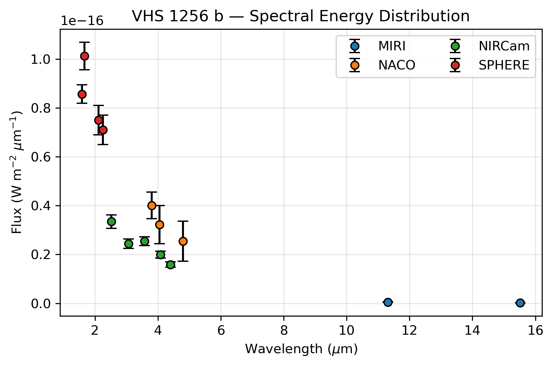
Number of photometric points: 14
Wavelength range: 1.59 - 15.51 µm

 WAV   WAVE_UNIT       FLX              ERR        RES   FAC    INS        FILT
------ --------- ---------------- ---------------- --- ------- ------ -------------
1.5888        um  8.569233656e-17 3.8338054057e-18   0 Paranal SPHERE IRDIS_D_H23_2
1.6671        um 1.0129485005e-16 5.6438364192e-18   0 Paranal SPHERE IRDIS_D_H23_3
  2.11        um          7.5e-17            6e-18   0 Paranal SPHERE IRDIS_D_K12_1
 2.251        um          7.1e-17            6e-18   0 Paranal SPHERE IRDIS_D_K12_2
 2.523        um        3.345e-17        2.714e-18   0    JWST NIRCam         F250M
 3.067        um        2.441e-17        1.868e-18   0    JWST NIRCam         F300M
  3.58        um        2.549e-17        1.785e-18   0    JWST NIRCam         F356W
   3.8        um    4.0100929e-17 5.4204869971e-18   0 Paranal   NACO            Lp
  4.05        um         3.22e-17          7.8e-18   0 Paranal   NACO         NB405
 4.084        um        1.989e-17        1.412e-18   0    JWST NIRCam         F410M
 4.397        um        1.589e-17        1.142e-18   0    JWST NIRCam         F444W
   4.8        um    2.5493937e-17          8.2e-18   0 Paranal   NACO            Mp
11.307        um        5.174e-19        8.038e-20   0    JWST   MIRI        F1140C
15.514        um         1.72e-19        2.897e-20   0    JWST   MIRI        F1550C
[6]:
fig, ax = plt.subplots(figsize=(6, 4), dpi=300)

# Plot each point with error bars, colored by instrument
grouped = table.group_by("INS")
for group in grouped.groups:
    inst_name = group["INS"][0]  # Get instrument name from first row of group
    mask = table["INS"] == inst_name
    ax.errorbar(wav[mask], flx[mask], yerr=err[mask], fmt="o", mec="k", ecolor="k", capsize=4, label=inst_name)

ax.set_xlabel(r"Wavelength ($\mu$m)")
ax.set_ylabel(r"Flux (W m$^{-2}$ $\mu$m$^{-1}$)")
ax.set_title("VHS 1256 b — Spectral Energy Distribution")
ax.grid(alpha=0.3)
ax.legend(ncols=2)
plt.tight_layout()
plt.show()
Section 3: Configure the analysis#
Part A: Setting up the configurations#
ForMoSA v2.0 uses four Python dataclasses to configure a run. Each dataclass groups related settings — you only need to set the ones that differ from the defaults.
Dataclass |
Controls |
|---|---|
|
File paths (observation, grid, output directories) |
|
How the grid is resampled to match the observations |
|
Wavelength fitting window, nested sampling algorithm |
|
Prior on each free parameter |
|
Settings for Nested Sampling Algorithms |
[7]:
from ForMoSA.config.global_config import ConfigPath, ConfigAdapt, ConfigInversion, ConfigParameters, Config_NS

# ──────────────────────────── Paths ────────────────────────────
config_path = ConfigPath(
    observation_path=[str(DATA_FILE)],          # list of FITS files
    adapt_store_path=str(TUTORIAL_DIR / "adapted_grid"),
    result_path=str(TUTORIAL_DIR / "results"),
    model_path=str(GRID_FILE),
)

# ────────────────────────── Adaptation ──────────────────────────
# Defaults are fine for photometry: no continuum removal (res_cont="NA"),
# target resolution = observation resolution (target_res_obs="obs").
config_adapt = ConfigAdapt(
        n_jobs = 12              # parallelize adaptation across 12 CPU cores (adjust as needed for your machine)
)

# ────────────────────────── Inversion ──────────────────────────
config_inversion = ConfigInversion(
    wav_fit   = ["2.0, 16.0"],   # µm range covering all 14 filters
    ns_algo   = "pymultinest",   # using pymultinest
    npoints   = 100,             # live points (increase for production runs)
    logL_type = ["chi2"],        # standard χ² likelihood
)

# ────────────────────────── Parameters ──────────────────────────
# Syntax for priors: ["type", "min", "max"] or ["constant", "value"]
# par1 = Teff (K), par2 = log g (dex) — read from grid attributes above
config_params = ConfigParameters(
    par1  = ["uniform", "400", "2000"],     # Teff range from BT-Settl grid
    par2  = ["uniform", "3.0", "5.0"],      # log g range
    par3 = ["uniform", "-0.5", "1.0"],       # metallicity [Fe/H] range (ExoREM grid only; ignored for BT-Settl)
    par4 = ["uniform", "0.1", "0.8"],        # C/O range (ExoREM grid only; ignored for BT-Settl)

    # r     = ["uniform", "0.5", "2.0"],      # radius (R_Jup)
    # d     = ["constant", "21.15"]           # distance (pc) — fixed to literature value for VHS 1256 b (21.15 ± 0.22 pc)
)

# ───────────────────── Nested Sampling Algo ───────────────────────
# Initialize the nested sampling configuration with the chosen algorithm (here, pymultinest)
config_ns = Config_NS()


# Display the configuration for verification
print("Configuration:")
print(f"  wav_fit : {config_inversion.wav_fit[0]} µm")
print(f"  Free    : {config_params.par1[1]} - {config_params.par1[2]} (Teff),"
      f" {config_params.par2[1]} - {config_params.par2[2]} (log g),"
      f" {config_params.par3[1]} - {config_params.par3[2]} ([M/H]),"
      f" {config_params.par4[1]} - {config_params.par4[2]} (C/O),"
      )
Configuration:
  wav_fit : 2.0, 16.0 µm
  Free    : 400 - 2000 (Teff), 3.0 - 5.0 (log g), -0.5 - 1.0 ([M/H]), 0.1 - 0.8 (C/O),
Saving the configuration for later reference#
[8]:
# Saving the configuration for later reference
from ForMoSA.config.global_config import ConfigGenerator

# Initialize the generator
generator = ConfigGenerator()

# Create a dictionary of your configuration objects
generator.config.update({
    "config_path": config_path,
    "config_adapt": config_adapt,
    "config_inversion": config_inversion,
    "config_parameters": config_params,
})

# Save to an .ini file
generator.save(path=TUTORIAL_DIR, name="photo_config.ini")
INFO Save config to path /Users/rajpoot/Karmabhumi/Packages/ForMoSA/docs/tutorials/photo/vhs1256b
Loading of the configuration file#
If you would like to use an already generated configuration file, then you have to load it first so that it can be passed to all algorithms. The Nested Sampling class will use only the parameters relevant to the algorithm you are using.
[9]:
from ForMoSA.config.global_config import ConfigLoader, Config_NS

# Load the configuration from the .ini file we just saved
cfg = ConfigLoader(str(TUTORIAL_DIR/'photo_config.ini'))
sections = cfg.load()

config_path = sections.get("config_path")
config_adapt = sections.get("config_adapt")
config_inversion = sections.get("config_inversion")
config_params = sections.get("config_parameters")

# Initialize Config_NS with the loaded configuration sections
config_ns = Config_NS(
                nestle=cfg.config['config_nestle'],
                pymultinest=cfg.config['config_pymultinest'],
                ultranest=cfg.config['config_ultranest']
            )
INFO Config file loaded
Step B: Setting up the Analysis object#
Analysis object is the main interface to run the ForMoSA using the provided configuration. It allows you to run the adaptation and inversion steps, or skip them if already done, and proceed directly to plotting results.
[10]:
from ForMoSA import Analysis

# If this is the first time you are adapting your model grid, or if you need to re-adapt it, set adapted = False
# If you have already adapted your model grid, set adapted = True
adapted = True

# If you want to perform the fit, set fitted = False
# If you only want to generate plots, set fitted = True
fitted = False

analysis = Analysis(config_path, adapted=adapted, fitted=fitted, log_level='ERROR')
INFO Filter data for Paranal/SPHERE.IRDIS_D_H23_2 successfully found
INFO Filter data for Paranal/SPHERE.IRDIS_D_H23_3 successfully found
INFO Filter data for Paranal/SPHERE.IRDIS_D_K12_1 successfully found
INFO Filter data for Paranal/SPHERE.IRDIS_D_K12_2 successfully found
INFO Filter data for JWST/NIRCam.F250M successfully found
INFO Filter data for JWST/NIRCam.F300M successfully found
INFO Filter data for JWST/NIRCam.F356W successfully found
INFO Filter data for Paranal/NACO.Lp successfully found
INFO Filter data for Paranal/NACO.NB405 successfully found
INFO Filter data for JWST/NIRCam.F410M successfully found
INFO Filter data for JWST/NIRCam.F444W successfully found
INFO Filter data for Paranal/NACO.Mp successfully found
INFO Filter data for JWST/MIRI.F1140C successfully found
INFO Filter data for JWST/MIRI.F1550C successfully found
INFO Setting wavelength unit to um for filter Paranal/SPHERE.IRDIS_D_H23_2 to um
INFO Setting wavelength unit to um for filter Paranal/SPHERE.IRDIS_D_H23_3 to um
INFO Setting wavelength unit to um for filter Paranal/SPHERE.IRDIS_D_K12_1 to um
INFO Setting wavelength unit to um for filter Paranal/SPHERE.IRDIS_D_K12_2 to um
INFO Setting wavelength unit to um for filter JWST/NIRCam.F250M to um
INFO Setting wavelength unit to um for filter JWST/NIRCam.F300M to um
INFO Setting wavelength unit to um for filter JWST/NIRCam.F356W to um
INFO Setting wavelength unit to um for filter Paranal/NACO.Lp to um
INFO Setting wavelength unit to um for filter Paranal/NACO.NB405 to um
INFO Setting wavelength unit to um for filter JWST/NIRCam.F410M to um
INFO Setting wavelength unit to um for filter JWST/NIRCam.F444W to um
INFO Setting wavelength unit to um for filter Paranal/NACO.Mp to um
INFO Setting wavelength unit to um for filter JWST/MIRI.F1140C to um
INFO Setting wavelength unit to um for filter JWST/MIRI.F1550C to um
NOTE: Here we create the main analysis class. For the purpose of not overcharging the notebook, we use log_level = ‘error’ The different options are:
‘info’ (basic information),
‘debug’ (basic information + additional debugging information)
‘warning’ (only warning messages)
‘error’ (only error messages, so typically no message unless you have an error in the code)
‘critical’ (same thing as ‘error’ but for critical ones)
‘off’ or None (no logging)
Section 4: Adapt the grid#
The grid is pre-computed at native model resolution. Before fitting, ForMoSA adapts it: it evaluates the model flux through each photometric filter, producing a much smaller grid of synthetic photometry that is directly comparable to your observations.
For photometry, adaptation is fast — there is no spectral convolution, just filter integration via the SVO Filter Profile Service (downloaded automatically the first time each filter is used).
Set adapted=True on subsequent runs to skip this step and load the cached grid.
[11]:
if not adapted:
    # Adaptation convolves each model spectrum to match the SINFONI resolution
    # and resamples it onto the observed wavelength grid.
    print("Adapting grid (convolution + resampling)...")
    analysis.adapt(config_adapt, config_inversion)
    print("Done. Set adapted=True to skip on re-runs.")
else:
    print("Skipping adaptation. Set adapted=False to re-run.")
Skipping adaptation. Set adapted=False to re-run.
Section 5: Run the nested sampling fit#
Nested sampling explores the prior volume and computes the Bayesian evidence (log Z) alongside the posterior distributions. In this tutorial, we will use pymultinest to run with more live points. This requires pymultinest to be installed locally. If not, then check the installation page for the instructions.
The npoints=100 setting is a good starting point for a quick check. For publication-quality posteriors, use 300–500 live points.
[12]:
if not fitted:
    print(f"Running {config_inversion.ns_algo} with {config_inversion.npoints} live points...")
    analysis.nested_sampling(config_params, config_adapt, config_inversion, config_NS=config_ns)
    print("\nFit complete. Results saved to results/")
else:
    print("Skipping fit. Set fitted=False to run the fit.")
Running pymultinest with 100 live points...
 *****************************************************
 MultiNest v3.10
 Copyright Farhan Feroz & Mike Hobson
 Release Jul 2015

 no. of live points =  100
 dimensionality =    4
 *****************************************************
 Starting MultiNest
 generating live points
 live points generated, starting sampling
Acceptance Rate:                        0.986842
Replacements:                                150
Total Samples:                               152
Nested Sampling ln(Z):               -399.659990
Importance Nested Sampling ln(Z):     -17.988714 +/-  0.729078
Acceptance Rate:                        0.862069
Replacements:                                200
Total Samples:                               232
Nested Sampling ln(Z):               -161.833011
Importance Nested Sampling ln(Z):     -18.375391 +/-  0.705344
Acceptance Rate:                        0.710227
Replacements:                                250
Total Samples:                               352
Nested Sampling ln(Z):                -88.807582
Importance Nested Sampling ln(Z):     -19.001596 +/-  0.600866
Acceptance Rate:                        0.704225
Replacements:                                300
Total Samples:                               426
Nested Sampling ln(Z):                -50.464958
Importance Nested Sampling ln(Z):     -19.663240 +/-  0.507255
Acceptance Rate:                        0.704225
Replacements:                                350
Total Samples:                               497
Nested Sampling ln(Z):                -33.893519
Importance Nested Sampling ln(Z):     -20.076692 +/-  0.414468
Acceptance Rate:                        0.709220
Replacements:                                400
Total Samples:                               564
Nested Sampling ln(Z):                -28.342425
Importance Nested Sampling ln(Z):     -19.979428 +/-  0.259031
Acceptance Rate:                        0.706436
Replacements:                                450
Total Samples:                               637
Nested Sampling ln(Z):                -24.937972
Importance Nested Sampling ln(Z):     -19.892256 +/-  0.172768
Acceptance Rate:                        0.682128
Replacements:                                500
Total Samples:                               733
Nested Sampling ln(Z):                -22.578561
Importance Nested Sampling ln(Z):     -19.756501 +/-  0.144845
Acceptance Rate:                        0.670732
Replacements:                                550
Total Samples:                               820
Nested Sampling ln(Z):                -21.102199
Importance Nested Sampling ln(Z):     -19.607520 +/-  0.114766
Acceptance Rate:                        0.643777
Replacements:                                600
Total Samples:                               932
Nested Sampling ln(Z):                -20.323562
Importance Nested Sampling ln(Z):     -19.533403 +/-  0.087153
Acceptance Rate:                        0.623202
Replacements:                                650
Total Samples:                              1043
Nested Sampling ln(Z):                -19.833876
Importance Nested Sampling ln(Z):     -19.452447 +/-  0.071253
Acceptance Rate:                        0.611354
Replacements:                                700
Total Samples:                              1145
Nested Sampling ln(Z):                -19.486608
Importance Nested Sampling ln(Z):     -19.372060 +/-  0.062748
Acceptance Rate:                        0.595238
Replacements:                                750
Total Samples:                              1260
Nested Sampling ln(Z):                -19.252171
Importance Nested Sampling ln(Z):     -19.333131 +/-  0.057736
Acceptance Rate:                        0.573066
Replacements:                                800
Total Samples:                              1396
Nested Sampling ln(Z):                -19.092126
Importance Nested Sampling ln(Z):     -19.325538 +/-  0.053433
Acceptance Rate:                        0.554107
Replacements:                                850
Total Samples:                              1534
Nested Sampling ln(Z):                -18.981997
Importance Nested Sampling ln(Z):     -19.320587 +/-  0.051424
Acceptance Rate:                        0.534759
Replacements:                                900
Total Samples:                              1683
Nested Sampling ln(Z):                -18.901294
Importance Nested Sampling ln(Z):     -19.314113 +/-  0.050354
Acceptance Rate:                        0.530029
Replacements:                                909
Total Samples:                              1715
Nested Sampling ln(Z):                -18.888969
Importance Nested Sampling ln(Z):     -19.311757 +/-  0.050188
 ln(ev)=  -18.707528226332368      +/-  0.21454620409313874
 Total Likelihood Evaluations:         1715
 Sampling finished. Exiting MultiNest
  analysing data from RAW_.txt

Fit complete. Results saved to results/
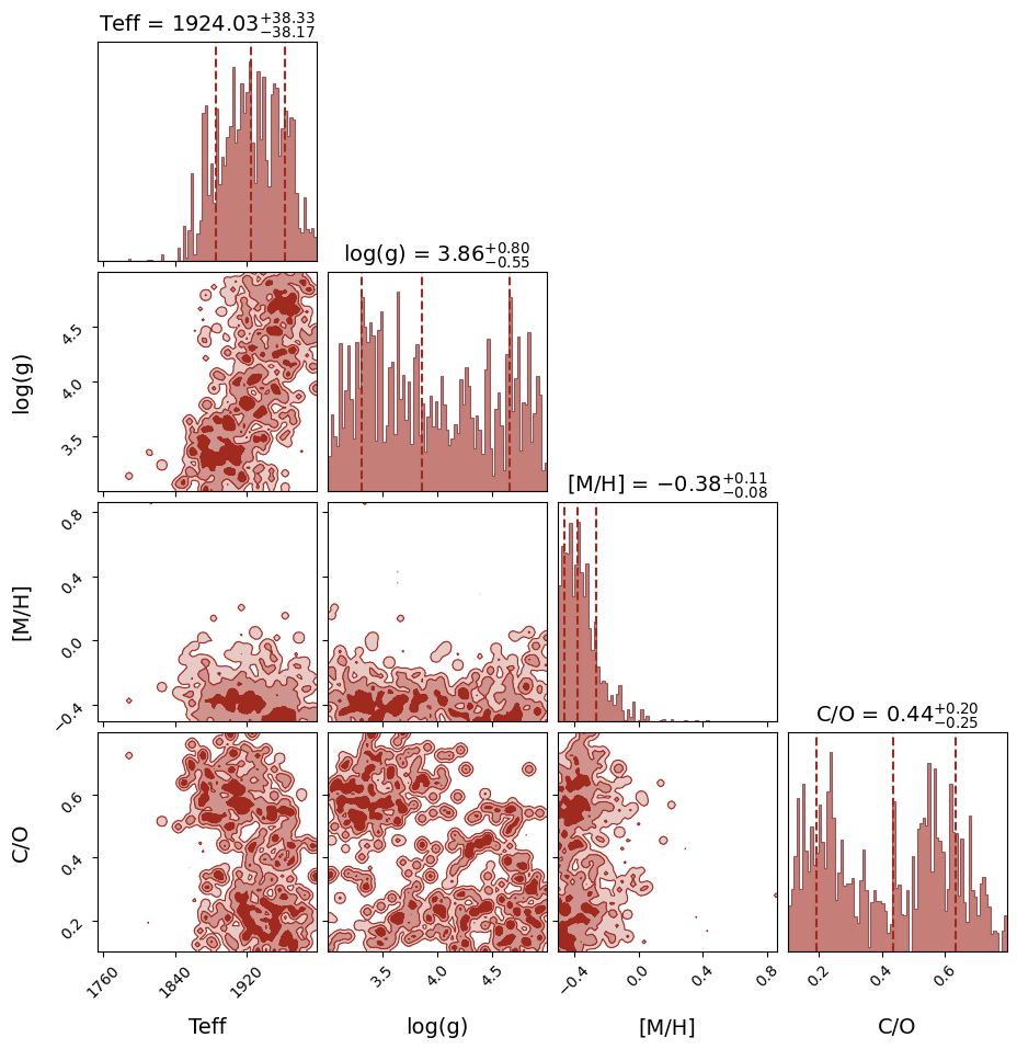
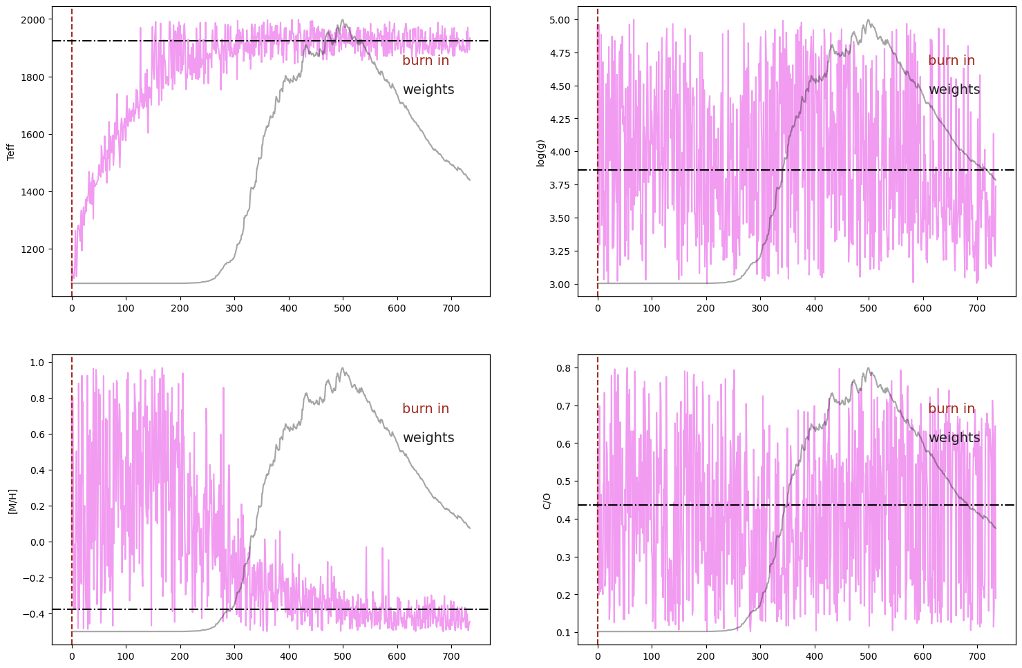
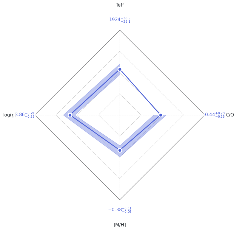
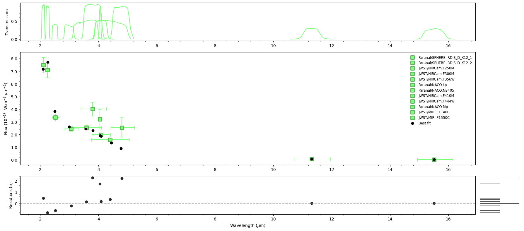
Section 6: Results#
ForMoSA produces four diagnostic plots saved to results/:
File |
Shows |
|---|---|
|
Posterior distributions and pairwise correlations |
|
Sample chains and weights (convergence check) |
|
Radar diagram of median ± 1σ for each parameter |
|
Best-fit model vs. observed data + residuals |
[13]:
# Plot all results
# The figures are also saved as PDFs in results/
analysis.plot(analysis.ns.results, plot_native_model=False)

# Print a numerical summary
print(analysis.ns.results.summary(sigma=1))
======== Nested Sampling Summary ====================
LogZ = -18.708 ± 0.215

Posterior estimates (median ± 1 sigma interval)

Teff        :  1923.9986 - 38.1410 + 38.4996 [1885.8576, 1962.4982]  MAP=1933.4565
log(g)      :     3.8596 -  0.5467 +  0.7947 [3.3129, 4.6544]  MAP=3.7371
[M/H]       :    -0.3763 -  0.0824 +  0.1139 [-0.4588, -0.2624]  MAP=-0.4444
C/O         :     0.4364 -  0.2459 +  0.1972 [0.1905, 0.6336]  MAP=0.1896
=====================================================
Section 7: INI file alternative#
The dataclass approach above is recommended — everything lives in one place and is easy to version-control. If you prefer an INI file (closer to ForMoSA v1.x and convenient for cluster runs), use ConfigGenerator to create a default template and ConfigLoader to load it.
[ ]:
from ForMoSA.config.global_config import ConfigGenerator, ConfigLoader, Config_NS

# 1. Generate a default config.ini in TUTORIAL_DIR
generator = ConfigGenerator()
generator.save(str(TUTORIAL_DIR), "config.ini")
print(f"Default config written to: {TUTORIAL_DIR / 'config.ini'}")
print("Open it in a text editor, fill in the paths and parameters, then load it:")
[ ]:
# 2. Load the config (after editing the .ini manually or programmatically)
# cfg = ConfigLoader(str(TUTORIAL_DIR / "config.ini"))
# sections = cfg.load()
#
# 3. Run — identical to the dataclass workflow:
# analysis = Analysis(cfg.config["config_path"], adapted=False, fitted=False)
# analysis.adapt(cfg.config["config_adapt"], cfg.config["config_inversion"])
# config_ns = Config_NS(
#     nestle=cfg.config["config_nestle"],
#     pymultinest=cfg.config["config_pymultinest"],
#     ultranest=cfg.config["config_ultranest"],
# )
# analysis.nested_sampling(
#     cfg.config["config_parameters"],
#     cfg.config["config_adapt"],
#     cfg.config["config_inversion"],
#     config_NS=config_ns,
# )
# analysis.plot(analysis.ns.results)
print("See the comments above for the full INI-based workflow.")
Section 8: Next steps#
Tutorial 2 — Spectroscopy (AB Pic b): Same adapt → sample → plot loop, but with a K-band spectrum. Introduces resolution adaptation and radial velocity.
Getting started guide:
docs/getting_started/config_file.mdfor a full parameter reference (prior types, MOSAIC indexing, HCHR options).API reference:
docs/api/for the full class and method documentation.
To fit your own target, copy this notebook and change:
DATA_FILE→ your.fitsobservation fileGRID_FILE→ your model grid (.nc)config_params→ priors appropriate for your target